| Shi-Keng Yang and Shuntai Zhou |
| RDC/Climate Prediction
Center/NCEP/NWS/NOAA |
| & |
| Alvin J. Miller |
| Climate Prediction
Center/NCEP/NWS/NOAA |
| Washington, DC 20233 |
|
ABSTRACT
In this paper, we describe a 3-D daily global ozone
analysis, Stratosphere Monitoring Ozone Blended Analysis (SMOBA), that is adopted for the
input to CERES/EOS heating rate calculation. The analysis can also be used for other
applications, such as the initial conditions for numerical ozone forecasts. The analysis
utilizes the operational SBUV/2 measurements blended with the total ozone measurements
from the 9.7 mm channel of HIRS/TOVS in the polar- night regions, where SBUV/2 data are
not available. Currently, both measurements are from the polar-orbiting satellite,
NOAA-14.
Monthly mean cross sections of ozone mixing ratio
for the period of March through June, 1997 are presented. As compared to the SBUV-only
climatology of Nagatani et al. (1988), SMOBA shows that ozone profiles in the polar
regions are a smooth extension from the sun-lit latitudes. An analysis of temporal
variations of mixing ratio is conducted for March and June. The results show that the
largest temporal variation are located in the lower stratosphere around 175 hPa for most
of the latitudes where the ozone concentration is the highest. In the upper stratosphere
from 30 hPa up, polar regions exhibit large seasonality, while the tropics remain fairly
calm. Spatial variations for Boreal equinox and solstice are also analyzed. Region-wise,
the results are very similar to the temporal variations. The implication from the results
of temporal and spatial variations is that without the dynamical effects, there could be
errors of heating rates were the zonal averaged climatology used in the radiative transfer
calculations in global numerical weather prediction models or general circulation models.
The vertical profiles of SMOBA are compared with
Microwave Limb Sounder (MLS). The results show that there is very good agreement in shape
and magnitude for the sun-lit northern hemisphere case. There is also reasonable agreement
with some characteristic differences for the southern hemisphere case. From 50o
S to 70o S, MLS profiles all peak at 5 hPa, while the SMOBA profiles peak from
8 hPa to 3 hPa. From 60o S to 80o S, SMOBA has higher magnitudes
between 5 hPa and 50 hPa. The higher magnitudes is very possibly caused from TOVS
overestimation of the total ozone.
1. Introduction :
Ozone has absorption features in both the solar (UV
band) and infrared (9.6 mm and 14 mm ) portions of the spectrum, and affects tropospheric
and stratospheric dynamics, radiation and chemistry. The vertical distribution of ozone
concentration is important in structuring the earth-atmospheric temperature profile. In a
sensitivity study, Ramanathan and Dickinson (1979) illustrate that the redistribution of
ozone profile imposes larger perturbation to the tropospheric fluxes than a uniform
changes of the profile. This finding implies that the recent ozone trend (Miller et al,
1995 and 1996), which occurs in the lower and upper stratosphere, can impose significant
forcing on the climate changes. Evaluating the possible impact, Lacis et al. (1990)
simulate a scenario of ozone change with a one-dimensional model. Their result found that
a decrease of ozone above ~30 km, and increase in tropospheric and lower stratospheric
ozone below ~30km, cause the global surface temperature to warm up. More recent experiment
with a general circulation model (GCM) by Ramaswamy et al (1996) also reports that the
ozone-induced cooling of the lower stratosphere leads to a negative radiative forcing of
the surface-troposphere system. As ozone is highly variable both in time and space, these
results indicate a need for a 3-dimensional (3-D) ozone analysis for studying the impacts
of ozone on the heating/cooling profiles in the atmosphere, and thus the climate.
The Stratosphere Monitoring Group at Climate
Prediction Center (CPC) / National Centers for Environmental Prediction (NCEP)/NWS/NOAA
has recently developed an algorithm for 3-D daily ozone analysis. The algorithm uses the
measurements from the Solar Backscatter Ultraviolet instrument (SBUV/2) (Bhartia, et al,
1996) which doesn't observe in the polar-night, blended with TOVS infrared ozone estimates
(Neuendorffer, 1996) in the regions of polar night to achieve global coverage. It is thus
called the Stratosphere Monitoring Ozone Blended Analysis (SMOBA). The current operational
polar-orbiting satellite, NOAA-14, contains both instruments. For its operational
stability and global coverage, SMOBA is adopted as the ancillary input data to the Cloud
and Earth Radiant Energy System (CERES) of EOS interdisciplinary study (Wielicki et al,
1996) which is to estimate atmospheric radiative divergence/ heating rates by utilizing
the meteorological, aerosol and ozone data from independent sources. CPC is also using
SMOBA as the initial conditions for experimental numerical forecast of ozone.
The selection of operational measurement of SBUV/2
and TOVS ozone as the basis for developing the SMOBA algorithm is prompted by the long
term stable global data stream required for supporting the CERES/EOS mission in studying
climate variation and climate changes. Although there have been a number of experimental
measurements that provide ozone profiles, such as and Cryogenic Limb Array Etalon
Spectrometer (CLAES) (Bailey et al, 1996), the Microwave Limb Sounder (MLS) (Froidevaux et
al, 1996), Improved Stratospheric and Mesospheric Sounder (ISAMS) (Connor et al, 1996) and
Halogen Occultation Experiment (HALOE) (Bruhl et al, 1996) onboard NASA Upper Atmosphere
Research Satellite (UARS), as well as Stratospheric Aerosol and Gas Experiment II (SAGE
II) (McCormick et al, 1989) on board NASA Earth Radiation Budget Satellite, none of the
above provides the global continuity of SBUV/2. TOVS total ozone is derived from the HIRS
9.7 mm channel, which can provide information for the regions which is not sun-lit. In
fact, the effective coverage of SBUV/2 is limited by the solar zenith angle of less
than.80o, which is a function of the satellites' equatorial crossing time.
Moreover, this blacked-out region tends to expands as the operational satellite precesses
to later equatorial crossing times. Hence we have formulated an algorithm, blending SBUV/2
and TOVS to add additional information for the polar-nights. Continuous daily SMOBA covers
the most comprehensive domain from surface to stratopause, from the pole to the pole.
This paper presents the procedure of SMOBA in
Section 2. Data analysis, which includes the monthly means and temporal and spatial
variations from the March to June 1997 is discussed in Section 3. Selected comparison with
the measurements from MLS/UARS is in section 4.
2. Data Analysis Algorithm:
The process of SMOBA starts from the orbital
information of the daily measurements of ozone mixing ratio and total column ozone that
are obtained from the NOAA polar orbiting satellite, currently NOAA-14. The retrieved
SBUV/2 ozone data include 19 levels of mixing ratio from 0.3 hPa to 100 hPa and total
column ozone. Layer ozone amounts are also included for 12 discrete layers from the
surface to ~60 km, but the vertical resolution is very coarse in the troposphere (only 2
layers).The input data are arranged along satellite orbit tracks, over the sun-lit portion
of the earth. We have performed objective analysis from the orbital data to a global, 2.5
x 2.5 degree latitude-longitude grid by a commonly used successive correction method (SCM)
(Daley, 1991). The output includes ozone mixing ratio at 24 pressure levels (0.2, 0.3,
0.4, 0.5, 0.7, 1, 1.5, 2, 3, 4, 5, 7, 10, 15, 20, 30, 40, 50, 70, 100, 150, 200, 250, 300
hPa) where we have added the 5 levels (300, 250, 200, 150, and 0.2 hPa) to the 19 level
input mixing ratio, which are derived from ozone amount data in layers 2 (256 - 128 hPa),
3 (128 - 64 hPa) and 12 (0.25 - 0.12 hPa) respectively. We also assume a uniform ozone
mixing ratio from 300 hPa to 1000 hPa, derived from the ozone amount in the lowest layer
(1000 - 256 hPa). The total ozone is directly from the retrieved data, which is the sum of
12 layer ozone amounts. Note that due to the different vertical resolution of the raw
data, the reliability of ozone mixing ratio is best above 30 hPa, good between 100 hPa and
30 hPa, and marginal below 100 hPa. We note, however, that the lower stratospheric ozone
retrievals are guided by climatology used in the ozone retrieval algorithm, and corrected
by the measured layer ozone amounts. The uniform tropospheric mixing ratio also captures
the main feature shown in ozone sonde measurements.
Because the SBUV/2 algorithm is based on the
sunlight absorbed and reflected by the atmosphere (iincluding ozone), there are no data in
polar night. To fill in the polar night gap, we use NOAA TOVS total ozone derived from
infrared measurements as the auxiliary information. However, TOVS does not measure
vertical ozone profiles. From other satellite data such as UARS MLS, CLAES, ISAMS and
HALOE, we have determined that the shapes of ozone vertical profiles are similar in polar
latitudes to those at high mid-latitudes. Therefore, we assume polar night ozone mixing
ratio to be such that its shape is the same as that of SBUV/2 ozone at the boundary of the
polar night, and the integrated polar total column ozone is equal to TOVS measurement. As
will be shown, this assumption is a reasonable approximation when the polar night gap is
not too large. Since TOVS total ozone is slightly different from SBUV/2 total ozone (~5%
at the boundary of polar night), a linear adjustment is applied to the polar ozone so that
the filled data joint smoothly at the boundary . This procedure is the so-called blended
data analysis, which combines the two data sources to obtain more complete information, on
the basis of physical and instrumental understanding. In operation, in case TOVS ozone is
not available for any reason, we simply use extrapolation to fill in the data gap.
Therefore, there are no gaps in the data analysis files.
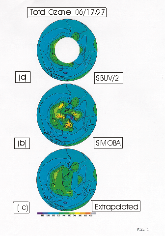
To demonstrate the effect of the blended analysis,
we show in Figure 1 example of total ozone maps in the southern hemisphere. Figure 1a is
SBUV/2 only for June 17, 1997. The polar night gap is near its winter solstice maximum,
and the data gap is even larger than the physical polar night region due to the time of
equatorial crossing, which is 1415 pm local time. In Figure 1b, TOVS data have been used
to fill the polar night gap, providing us with detailed polar ozone characteristics such
as wave patterns and a minimum at the east shore of Antarctica. The TOVS data has been
slightly adjusted according to the SBUV/2 data at the polar night edge, so that there are
no discontinuities or sharp gradients at the edge due to instrumental difference. As a
comparison Figure 1c shows SBUV/2 data with extrapolations into polar night gap.
Apparently, those real polar ozone features could not be reproduced due to relatively
large expanse of the polar night region. Fortunately, we have both SBUV/2 and TOVS in NOAA
operational satellites. Thus we do not have to extrapolate data in order to generate a
globally covered, 3-D near real time daily ozone field.
3. Results from the first four months
operation:
3.1 Monthly Means
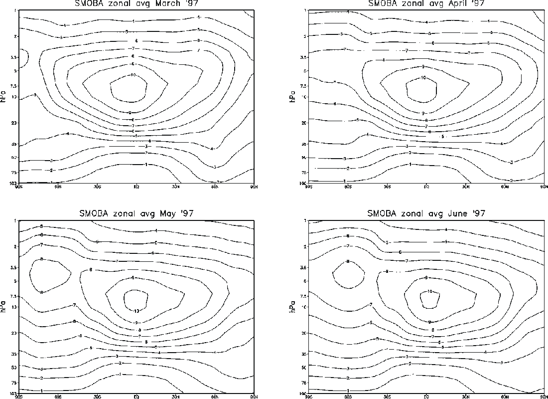
SMOBA began daily operation on March 1, 1997.
Figure 2 illustrates the monthly mean pressure-latitude cross sections for the first four
months. The general features of ozone cross section have a mixing ratio maximum located
near 8 hPa, about 33 km altitude. The maximum moves from 8o S in March
northward to about 5o N in June. The maxima of the vertical profiles raise
gradually from 8 hPa at equator to about 5 hPa at the poles. For May and June, there
exists a second maximum larger than 8 ppmv located at about 8 hPa and 60 S, which also
moves northward slightly from May to June. This result agrees very well with other
published SBUV atlases, such as Nagatani et al. (1988), which contains 8-year average SBUV
measurements for the sun-lit area and uses Cressman objective analysis (1959). SMOBA
expands the domain to include the regions of polar night, and this analysis demonstrates
that the cross section of ozone mixing ratio in the polar region is a smooth extension
from the sun-lit regions.
3.2 Temporal Variations :
Stratospheric ozone constitutes an important
greenhouse gas with substantial temporal and spatial variation that is not revealed in the
seasonal variation shown in Fig. 2. Significant temporal variations of ozone usually occur
in the day-to-day scale, which could be significant departures from the monthly
climatologies or monthly means. Fig. 3 depicts the standard deviations of the ozone mixing
ratio sampled from the daily analysis and normalized to the monthly means for March and
June 1997. This result is in contrast to the interannual variance shown in Nagatani et al.
(1988) which samples the monthly means from 8 years data. The normalization enhances the
significance of the variability in the lower stratosphere, between 150 hPa and 75 hPa,
where the ozone concentration is the highest.
The maximum of the normalized standard deviation
generally occurs around 125 hPa for most of the latitudes, and ranges from 9% to more than
24% for March (Fig. 3a). At this altitude, the maximum of the normalized standard
deviation occurs at 33 0 N with the intensity of 27%. Not mirroring the
northern hemisphere, southern hemisphere has a maximum of more than 15% at 45o
S. Although the features in the northern hemisphere is not symmetric to the southern
hemisphere from 30 hPa upward, there is a gradual poleward increase of normalized standard
deviation from 3% at 30o N and S to 9% at poles, while the tropics is quite
homogeneous.
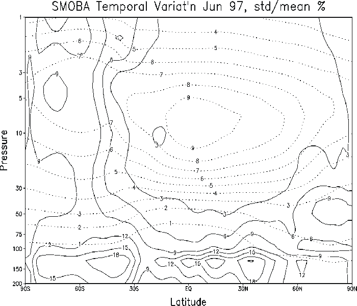
Fig. 3b shows the corresponding normalized standard
deviation for June. Albeit there exists similar synoptic features as March, the global
pattern is severely skewed toward the southern hemisphere, especially from 30 hPa upward.
The whole field from 30o S northward to the Arctic is very homogeneous. In the
lower stratosphere, the maximums are still located around 125 hPa for most of the
latitudes, and ranges from 9% to 21%.
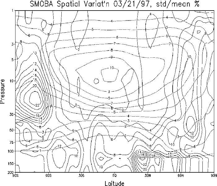
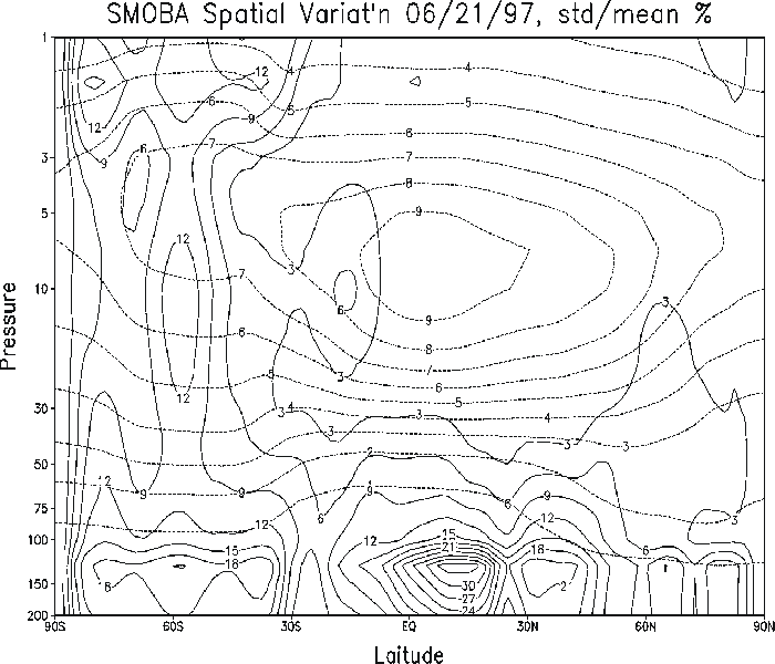
3.3 Spatial variations:
The boreal spring equinox and summer solstice are
selected for illustrating the deviation from the zonal means around the globe. Fig. 4 is
constructed by calculating the standard deviations about the zonal means normalized by the
zonal means. Region-wise the general global pattern of this figure somewhat resembles the
temporal variations of Fig. 3, with very homogeneous field in the tropics from 30 hPa
upward, i.e. the ozone distribution in this region is very zonal. At the lower
stratosphere, around 175 hPa, the normalized standard deviation has much larger magnitudes
ranges from 10% to 20% for the spring equinox, Fig. 4a. A maximum of 20% locates at 175
hPa, 27o N, is the largest in the lower stratosphere, while there are less
clearly defined maximums in the southern hemisphere at 15o S and around 55o
S with a magnitudes of 10%. Very distinctive from Fig. 4a is from 30 hPa upward at
southern polar region, where a well defined maximum of 20% is located at 20 hPa 70oS
with substantial gradients from the center. While there appears to be a similar maximum in
the northern hemisphere around 20 hPa 70o N with the intensity of 10%, it is
very mild.
On the boreal summer solstice, Fig. 4b, it appears
that the ozone distribution in both hemispheres are far from zonal in the lower
stratosphere from the tropics to the mid latitudes, particularly from the equator to 25o
N, where a maximum of 30% exists at 175 hPa. In the low latitudes, the mean zonal mixing
ratio is small, about 0.1 to 0.2 ppmv as compared to 0.6 ppmv for the polar regions. Thus,
any departure from the mean could be enhanced. From 30 hPa upward, most of the deviations
are in the southern hemisphere from 30o S poleward, while the northern
hemisphere is fairly zonal. The implication from the results of temporal and spatial
variations is that there could be errors of heating rates were the zonal averaged
climatology used in the radiative transfer calculations in global NWP models or general
circulation models.
4. Profile Comparison with MLS
Limited ozone profiles from Microwave Limb Sounder
(MLS) (Froidevaux, 1996) are available for comparison from UARS, which is in a 58o
inclined orbit. For this particular period under study, the UARS is operating under a
power deficiency, so that all instruments can not be on all the time. SAGEII, also, is
limited in coverage of the polar regions. Therefore, we have focused attention on the MLS
(Version 4) , which provides 2 days of comparision from April 1 (South facing) to April 10
(North facinging). The facing of UARS enable MLS to measure further poleward then the
terminator of orbital inclination. the MLS provides profiles from 100 hPa up with coarser
vertical resolution than SMOBA.
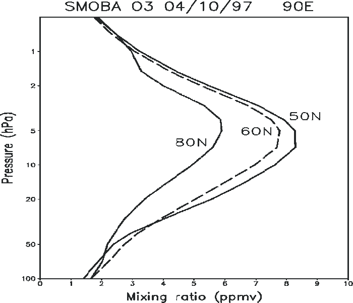
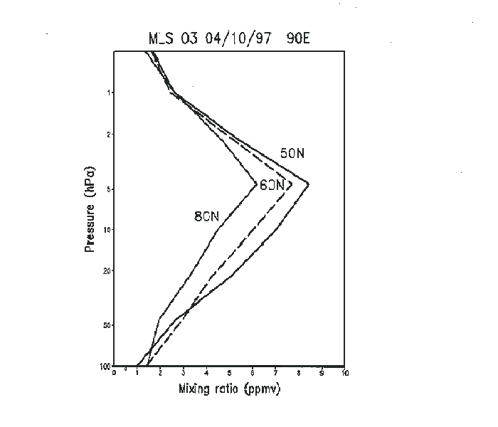
On April 10, 1997, the SMOBA profiles at three
locations, 90oE and 50o N, 60o N, and 80o N,
respectively, are on Fig. 5a. The corresponding MLS profiles are on Fig. 5b. This is a
case that SBUV/2 has coverage up to 80o N, thus most of the profiles are from
measurements instead of blending with TOVS ozone. It is clear that the higher resolution
of SMOBA makes the profiles smoother. Nevertheless, there is very good agreement as both
MLS and SMOBA have profiles peaks around 5 hPa for all the three locations. The magnitudes
of the peaks at 50oN (60oN) for SMOBA agree with that of MLS, within
0.2 (0.1) ppmv out of 8.4 (7.7) ppmv, while the one at 80oN differ slightly
larger, 0.5 ppmv out of 6.2 ppmv. Although there is precise agreement for the peak at 60oN,
profile-wise, SMOBA overestimates MLS from 20 hPa to 5 hPa with largest difference of 0.7
ppmv at 10 hPa. The profiles at the other two locations are in good agreement within 0.4
ppmv for all the altitudes. Although not shown, we have also compared similar profiles for
the same latitudes at 0o E, 180o, and 90o W. All of them
have the similar characteristics and good agreement.
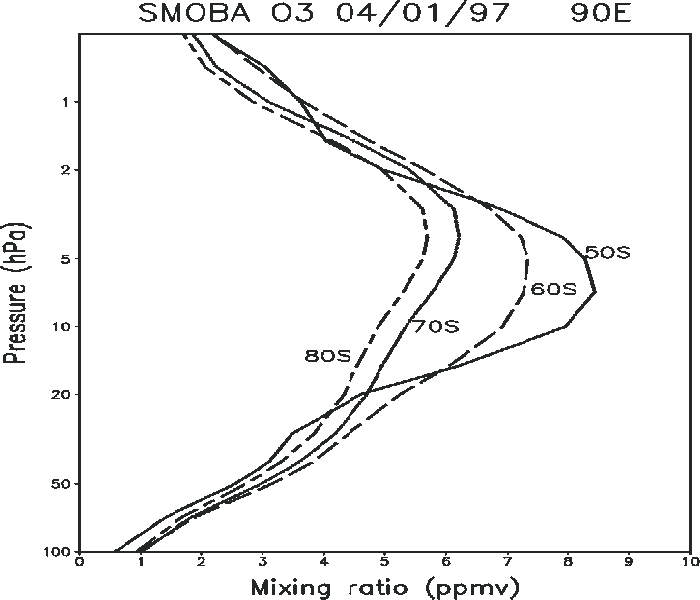
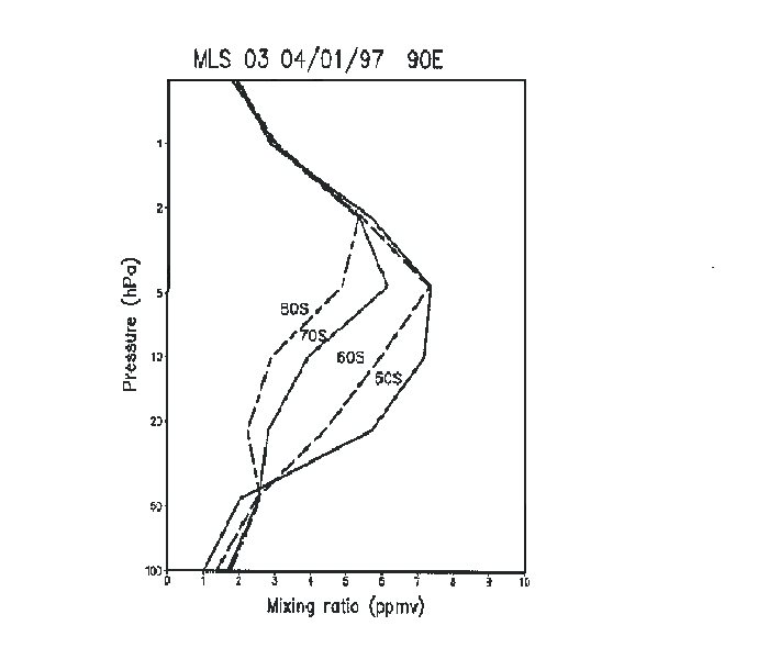
For the case in the southern hemisphere on April 1,
1997 at 90o W, SBUV/2 has coverage down to around 680 S. The SMOBA
profiles higher than 680 S, Fig. 5c, are from blending TOVS ozone, namely the
profiles at the boundary of the polar nights are carried into the higher latitudes.
For this reason, the shape of the profiles at 70o
S and 80o S are very similar. Comparison with MLS, Fig. 5d, shows that there is
quite reasonable agreement between the two data sets especially below 50 hPa and above 2
hPa, and with some characteristic differences in between. From 50o S to 70o
S, MLS profiles all peak at 5 hPa, while the SMOBA profiles peak from 8 hPa to 3 hPa. At
70o S and 80oS from 5 hPa to 50 hPa, SMOBA mixing ratio decreases
substaintially slower than that of MLS. Conversely is the case at 50o S from 15
hPa to 50 hPa. From 60o S to 80o S, SMOBA has higher magnitudes
between 5 hPa and 50 hPa. Integrating the column ozone from 100 hPa to 1 hPa found that
SMOBA is about 10 % higher than MLS from 60oS poleward. Although there has been
few studies on the polar night ozone profiles, the most reasonable conjecture for the
cause of this difference is possibly from the overestimates of the total ozone by TOVS.
Table 2 of Neuendorffer (1996) documents "Auxiliary TOVS Total Ozone
Adjustments" derived from comparison with total ozone-mapping spectrometer (TOMS)
between 75o S and 75o N. For mean April difference averaged from
1979 through 1992, it states that TOVS is 36 Dobson Unit higher than TOMS. To comply with
TOMS, it is possible in the future to develop a similar daily table for adjustment once
SMOBA has collected a full year data. The adjustment can narrow the gap between SMOBA and
MLS. However, it can not change the shape of SMOBA profiles in polar-nights, which calls
for further research.
Summary:
For computing global heating rate, CERES/EOS has
adopted a 3-D daily global ozone analysis, SMOBA, as an ancillary input. The analysis
developed at CPC/NCEP employes a successive correction method and uses operational SBUV/2
measurements in the sun-lit regions, blended with the total ozone measurements from the
9.7 mm channel of HIRS/TOVS in the polar- night regions. Currently, both measurements are
from the polar-orbiting satellite, NOAA-14. This near real-time analysis can also be used
for other applications, such as the initial conditions for numerical ozone forecasts that
CPC/NCEP is experimenting.
Since began daily operation on March 1, 1997, SMOBA
has proven itself to be a very stable and reliable algorithm required by the coming CERES
operations. Monthly mean cross sections of ozone mixing ratio for the period of March
through June, 1997 are presented. As compared to the SBUV-only climatology of Nagatani et
al. (1988), which uses Cressman objective analysis, SMOBA shows that ozone profiles in the
polar regions are a smooth extension from the sun-lit latitudes. The maximum of the ozone
mixing ratio located near 8 hPa and moves from 8o S in March northward to about
5o N in June. An analysis of temporal variations of mixing ratio is conducted
for March and June. The results show that the largest temporal variation are located in
the lower stratosphere around 175 hPa for most of the latitudes where the ozone
concentration is the highest. In the upper stratosphere from 30 hPa up, polar regions
exhibit large seasonality, while the tropics remain fairly calm. Spatial variations for
Boreal equinox and solstice are also analyzed. Region-wise, the results are very similar
to the temporal variations. The implication from the results of temporal and spatial
variations is that without the dynamical effects, there could be errors of heating rates
were the zonal averaged climatology used in the radiative transfer calculations in global
numerical weather prediction models or general circulation models.
Two cases of the SMOBA vertical profiles are
compared with the measurements from MLS (Version 4) onboard UARS, one case for each
satellite facing, respectively. The results show that there is very good agreement in
shapes and magnitudes for the sun-lit northern hemisphere case (South facing), April 10,
1997. There is also reasonable agreement with some characteristic differences for the
southern hemisphere case (North facing), April 1, 1997. From 50o S to 70o
S, MLS profiles all peak at 5 hPa, while the SMOBA profiles peak from 8 hPa to 3 hPa. From
60o S to 80o S, SMOBA has higher magnitudes between 5 hPa and 50
hPa. The higher magnitudes is very possible caused from TOVS overestimation. Adjustment at
high latitudes can be developed once SMOBA collects one full year data. Since there are
limited ozone profiles available for polar night, the result calls for more research
before adjustment to the shape of profile can be made.
For further studying the profiles of polar nights,
it is our intent to analyze July and December '97 data in the future when they are
available. A comparison with MLS or other ozone sonde measurements can be conducted.
SMOBA started the routine operation on March 1,
1997. A ten-day rotating file has been set up for anonymous FTP at:
ftp.cpc.ncep.noaa.gov/SMOBA/.
Acknowledgment:
This work is supported by a NASA Langley Research
Center Grant L90988C. Discussions with Drs. Ron Nagatani, Hai-Tien Lee, Craig Long and Mel
Gelman have been very helpful.
References:
Bailey, P. L., D. P. Edwards, J. C. Gille, L. V.
Lyjak, S. T. Massie, A. E. Roche, J. B. Kumar, J. L. Mergenthaler, B. J. Connor, M. R.
Gunson, J. J. Margitan, I. S. McDermid, and T. J. McGee, Comparison of cryogenic limb
array etalon spectrometer (CLAES) ozone observations with correlative measurements, J.
Geophy. Res., 9737-9756, 1996.
Bhartia, P. K., R. D. McPeters, C. L. Mateer, L. E.
Flynn, and C. Wellemeyer, Algorithm for the estimation of vertical ozone profiles from the
backscattered ultraviolet technique, J. Geophy. Res., 101, No. D13, 18793-18806, 1996.
Bruhl, C., S. R. Drayson, J. M. Russell III, P. J.
Crutzen, J. M. McInerney, P. N. Purcell, H. Clande,, H. Gernandt, T. J. McGee, I. S.
McDermid, and M. R. Gunson, Halogen Occulatation Experiment ozone channel validation, J.
Geophys. Res., 10217-10240, 1996.
Connor, B. J., C. J. Scheuer, D. A. Chu, J. J.
Remedios, R. G. Grainger, C. D. Rogers, and F. W. Taylor, Ozone in the middle atmosphere
as measured by the improved stratospheric and mesospheric sounder, J. Geophys. Res.,
9831-9842, 1996.
Cressman, G. P., An Operational Objective Analysis
System, Mon. Wea. Rev., 87 No. 10, 367-374, 1959.
Daley, R., Atmospheric Data Analysis, Cambridge
University Press, 457pp, 1991
Froidevaux, L., W. G. Read, T. A. Lungu, R. E.
Cofield, E. F. Fishbein, D. A. Flower, R. F. Jarnot, B. P. Ridenoure, Z. Shippony, J. W.
Waters, J. J. Margitan, I. S. McDermid, R. A. Stachnik, G. E. Peckham, G. Braathen, T.
Deshler, J. Fishmanm, D. J. Hofmann, and S. J. Oltmans, Validation of UARS Microwave Limb
Sounder ozone measurements, J. Geophy. Res., 10017-10060, 1996
Lacis, A. A., D.J. Wuebbles, J. A. Logan, Radiative
forcing of climate by changes in the vertical distribution of ozone, J. Geophy. Res., 95,
No. D7, 9971-9981, 1990.
McCormick, M. P., J. M. Zawodny, R. E. Veiga, J. C.
Larsen, and P. H. Wang, An overview of SAGE I and II ozone measurements, Planet. Space
Sci., 37 No.12, 1567-1586. 1986
Miller, A. J., G. C. Tiao, G.C. Reinsel, D.
Wuebbles, L. Bishop, J. Kerr, R. M. Nagatani, J. J. DeLuisi, and C. L. Mateer, Comparisons
of observed ozone trends in the stratosphere through examination of Umkehr and ballon
ozonesonde data, J. Geophy. Res., 100, N. D6, 11209-11217, 1995.
Miller, A. J., S. M. Hollandsworth, L.E. Flynn,
G.C. Tiao, G.C. Reinsel, L. Bishop, R. D. McPeters, W. G. Planet, J. J. Deluisi, C. L.
Mateer, D. Wuebbles, J. Kerr, and R. M. Nagatani, Comparisons of observed ozone trends and
solar effects in the stratosphere through examinatio of ground-based Umkehr and combined
solar backscattered ultraviolet (SBUV) and SBUV2 satellite data, J. Geophy. Res., 101, No
C4, 9017-9021, 1996.
Nagatani, R.M., A. J. Miller, K. W. Johnson, and
M.E. Gelman, An eight-year climatology of meteorological and SBUV ozone data, NOAA Tech.
Report, NWS40. U.S. Dept of Commerce, 125pp, 1988.
Neuendorffer, A.C., Ozone monitoring with TIROS-N
operation vertical sounders, J. Geophy. Res., 101, No. D13, 18807-18828, 1996.
Ramanathan, V. and R. E. Dickinson, The Role of
Stratospheric Ozone in the Zonal and Seasonal Radiative Energy Balance of the
Earth-Troposhere System, J. Atmos. Sci., 36, 1084-1104, 1979.
Ramaswamy,V., M. D. Schwarzkoph and W. J. Randel,
Fingerpirnt of ozone depletion in the spatial and temporal pattern of recent
lower-stratospheric cooling. Nature, 382, 616-618, 1996.
Wielicki, B. A., B. R. Barkstrom, E. F. Harrison,
R. B. Lee, G. L. Smith and J. E. Copper, Clouds and the Earth's Radiant Energy System
(CERES): An Earth Observing System Experiment, Bull. Amer. Meteo. Soc., 77, 853-868, 1996.
Figure Caption:
Fig. 1: Total column ozone
for June 17, 1997, in Dobson Unit. (a) Analysis of SBUV/2 without fill-in for polar night;
(b) SMOBA; (c) Fill in polar night of (a) by simple extrapolation.
Fig. 2: Monthly mean cross
sections of ozone mixing ratio for March , upper left panel; April, upper right panel;
May, lower left panel, and June 1997, lower right panel, in ppmv. Contour interval is 1
ppmv.
Fig. 3a: SMOBA temporal
variation for March, 1997. The thick lines are the standard deviations from daily ozone
mixing ratio divided by the monthly mean, in %. contour interval is 3%. The thin lines are
the contours of monthly mean ozone mixing ratio as in Fig. 2, in ppmv. Contour interval is
1 ppmb. The ordinate is height in hPa.
Fig. 3b: same as Fig. 3a,
but for June, 1997.
Fig. 4a: SMOBA spatial
variation for March 21, 1997. The thick lines are the standard deviations of ozone mixing
ratio divided by the zonal mean, in %. contour interval is 3%. The thin lines are the
contours of zonal mean ozone mixing ratio, in ppmv. Contour interval is 1 ppmb. The
ordinate is height in hPa.
Fig. 4b: Same as Fig. 4a,
but for June 21, 1997.
Fig. 5a: SMOBA Ozone
profiles at (50o N, 90oE), (60o N, 90oE) and
(80o N, 90oE) for April 10, 1997, in ppmv
Fig. 5b: Same as Fig. 5a,
but from MLS.
Fig. 5c: SMOBA Ozone
profiles at (50o S, 90oW), (60o S, 90oW) and
(80o S, 90oW) for May 19, 1997, in ppmv
Fig. 5d: Same as Fig. 5c,
but from MLS.
|


